Explore Tensorflow features with the CIFAR10 dataset

The reason I started using Tensorflow was because of the limitations of my experiments so far, where I had coded my models from scratch following the guidance of the CNN for visual recognition course.

I already knew how CNN worked, and had already a good experience of what it takes to train a good model. I had also read a lot of papers presenting multiple variations of CNN topologies, those aiming at increasing accuracy like those aiming at reducing model complexity and size.

I work in the embedded world, so performance is obviously one of my primary concern, but I soon realized that the CNN state of the art for computer vision had not reached a consensus yet on the best compromise between accuracy and performance.

In particular, I noticed that some papers had neglected to investigate how the multiple characteristics of their models contribute to the overall results they obtain: I assume that this is because it takes an awful lot of time to train a single model, thus leaving no time for musing around.

Anyway, my goal was therefore to multiply experiments on several models to better isolate how each feature contributes to the efficiency of the training and to the performance of the inference.

More specifically, my goals were:

• to verify that Tensorflow allowed me to improve the efficiency of my trainings (going numpy-only is desperately slow, even with BLAS and/or MKL),
• to use this efficiency to multiply experiments, changing one model parameter at a time to see how it contributes to the overall accuracy,
• to experiment with alternative CNN models to verify the claims in the corresponding papers.

Thanks to the CNN for visual recognition course, I had already used the CIFAR10 dataset extensively, and I was sure that its complexity was compatible with the hardware setup I had.

I therefore used the tensorflow CIFAR10 image tutorial as a starting point.

Setting up a Tensorflow environment

I have a pretty good experience in setting up development environments, and am very much aware of the mess your host system can become if you don’t maintain a good isolation between these developments environments.

After having tried several containment techniques (including chroots, Virtual Machines and virtual env), I now use docker, like everybody else in the industry.

Google provides docker images for the latest Tensorflow versions (both CPU and GPU), and also a development image that you can use to rebuild Tensorflow with various optimizations for your SoC.

You can refer to my step by step recipe to create your environment using docker.

Creating a CIFAR10 training framework

Taking the Tensorflow image tutorial as an inspiration, I developed a generic model training framework for the CIFAR10 dataset.

The framework uses several types of scripts for training and evaluations.

All scripts rely on the same data provider based on the tensorflow batch input pipeline.

The training scripts uses Tensorflow monitored training sessions, whose benefits are twofolds:

• they neatly take care of tedious tasks like logs, saving checkpoints and summaries,
• they almost transparently give access to the Tensorflow distributed mode to create training clusters.

There is one script for training on a single host and another one for clusters.

There is also a single evaluation script, and a script to ‘freeze’ a model, ie combine its graph definition with its trained weights into a single model file that can be loaded by another Tensorflow application.

I tested the framework on a model I had already created for the assignments of my course, verifying that I achieved the same accuracy.

The framework is in this github repository.

Reproducing the tutorial performance

The next step was to start experimenting to figure out what really matters in a CNN model for the CIFAR10 dataset.

The idea was to isolate the specific characteristic of the tutorial model to evaluate how they contribute to the overall model accuracy.

As a first step, I implemented the same model as the tutorial in my framework, but without all training bells and whistles.

Basic hyperparameters

Learning rate and batch size are two of the most important hyperparameters, and are usually well evaluated by model designers, as they have a direct impact on model convergence.

So I would assume they are usually well-defined. I nevertheless tried different training parameters, and finally decided to keep the ones provided by the tutorial, as they gave the best results:

• learning rate = 0.1,
• batch size = 128.

Note: the learning rate is more related to the model, and the batch size to the dataset.

Initialization

For the initialization parameters, I was a bit reluctant to investigate much, as there were too many variations.

More, I had already tried the Xavier initialization with good success, so I decided to initialize all variables with a Xavier initializer.

weight decay

For the weight decay, I used a global parameter for each model, but refined each for each variable, dividing it by the matrix size: my primary concern was to make sure that the induced loss did not explode.

Gradually improving from my first results

With my basic setup, I achieved results a bit lower than the tutorial (for exactly the same model):

75,3 % accuracy after 10,000 iterations instead of 81,3%.

Then, I added data augmentation, that smoothed a lot the training process:

• drastic reduction of the overfitting,
• lower results for early iterations,
• much higher results after 5000+ iterations.

With data augmentation:

78,8 % accuracy after 10,000 iterations.

Finally, I used trainable variables moving averages instead of raw values, and it gave me the extra missing accuracy to match the tutorial performance:

81,4% accuracy after 10,000 iterations.

After 300,000 iterations, the model with data augmentation even reached 87% accuracy.

Conclusion

For the CIFAR10 dataset, data augmentation is a key factor for a successful training, and using variable moving averages ireally helps convergence.

Tutorial model metrics

Without data augmentation (32x32x3 images):

Size  : 1.76 Millions of parameters
Flops : 66.98 Millions of operations

With data augmentation (24x24x3 images):

Size     : 1.07 Millions of parameters
Flops    : 37.75 Millions of operations

Experimenting with the tutorial model topology

To better understand how the tutorial model topology, I tested a few ALexNet-style models variants.

Note: I call these models Alex-like as the tutorial is based on the models defined by Alexei krizhevsky, winner of the ImageNet challenge in 2012).

I didn’t save all variants I tried, but to summarize my experiments:

• Local-response-normalization is useless,
• One of the FC layer can be removed without harming accuracy too much,
• For the same amount of parameters, more filters with smaller kernels are equivalent to the base setup.

My conclusion is that the tutorial model can be improved a bit in terms of size and processing power (see the Alex 4 variant for instance), but that it is already a good model for that specific topology that combines two standard convolutional layers with two dense layers.

Experimenting with alternative models

The next step was to experiment further with different models:

• NiN networks that remove dense layers altogether,
• SqueezeNets that parallelize convnets.

The idea was to stay within the same range in terms of computational cost and model size, but trying to find a better compromise between model accuracy, model size and inference performance.

The figure below provides accuracy for the three best models I obtained, compared to the tutorial version and one of the Alex-style variant.

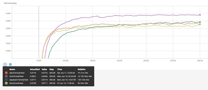
For each model, I evaluated the model size in number of parameters, and its computational cost in number of operations.

To put these theoretical counters in perspective, I also got ‘real’ numbers by checking:

• the actual disk size of the saved models,
• the inference time using the C++ label_image tool (I added some traces)

The ratio between the number of parameters and the actual size on disk seems consistent for all models, but the inference time is not, and may vary greatly depending on the actual local optimizations. The winner is however the model with the less number of operations.

Here are the detailed numbers for all trained models :

Tuto

Accuracy : 87,2%
Size     : 1.07 Millions of parameters  / 4,278,750 bytes
Flops    : 37.75 Millions of operations / 44 ms

Alex (alex4)

Accuracy : 87,5%
Size     : 1.49 Millions of parameters  / 5,979,938 bytes
Flops    : 35.20 Millions of operations / 50 ms

NiN (nin2)

Accuracy : 89,8%
Size     : 0.97 Millions of parameters   / 3,881,548 bytes
Flops    : 251.36 Millions of operations / 90 ms

SqueezeNet (squeeze1)

Accuracy : 87,8%
Size     : 0.15 Millions of parameters   / 602,892 bytes
Flops    : 22.84 Millions of operations  / 27 ms

Conclusion

From all model topologies I studied here, the SqueezeNet architecture is by far the most efficient, reaching the same level of accuracy with a model that is more than six times lighter than the tutorial version, and more than 1,5 times faster.

Further experiments

In my alternative models, I had first included Inception, but I ruled it out after finding out how NiN was already costly: it would nevertheless be interesting to evaluate Xception, one of its derivative that uses depthwise separable convolutions.

Last, I would like to check how these models could be compressed using iterative pruning and quantization.