Simulating spiking neurons with Tensorflow

Spiking Neural Networks are the next generation of machine learning, according to the litterature.

After the feed-forward perceptrons of the last century and the bi-directional deep networks trained using gradient descent of today, this 3rd generation of neural networks uses biologically-realistic models of neurons to carry out computation.

A spiking neural network (SNN) operates using spikes, which are discrete events that take place at points in time, rather than continuous values. The occurrence of a spike is determined by differential equations that represent the membrane potential of the neuron. Essentially, once a neuron reaches a certain potential, it spikes, and the potential of that neuron is reset.

In this article, I will detail how this kind of network can be modelled using Tensorflow.

You can find a jupyter notebook corresponding to this article in my tensorflow sandbox.

The article is based on an existing exercise using Matlab.

Spiking neuron model

The neuron model is based on “Simple model on spiking neuron”, by Eugene M. Izhikevich.

Electronic version of the figure and reproduction permissions are freely available at www.izhikevich.com

The behaviour of the neuron is determined by its membrane potential v that increases over time when it is stimulated by an input current I. Whenever the membrane potential reaches the spiking threshold, the membrane potential is reset.

The membrane potential increase is mitigated by an adversary recovery effect defined by the u variable.

Tensorflow doesn’t support differential equations, so we need to approximate the evolution of the membrane potential and membrane recovery by evaluating their variations over small time intervals dt:

We can then apply the variations by multiplying by the time interval dt:

As stated in the model, the $0.04$, $5$ and $140$ values have been defined so that $v$ is in $mV$, $I$ is in $A$ and $t$ in $ms$.

The corresponding Tensorflow code looks like this (see the jupyter notebook for details):

# Evaluate membrane potential increment for the considered time interval
# dv = 0 if the neuron fired, dv = 0.04v*v + 5v + 140 + I -u otherwise
dv_op = tf.where(has_fired_op,
                 tf.zeros(self.v.shape),
                 tf.subtract(tf.add_n([tf.multiply(tf.square(v_reset_op), 0.04),
                                       tf.multiply(v_reset_op, 5.0),
                                       tf.constant(140.0, shape=[self.n]),
                                       i_op]),
                             self.u))
                        
# Evaluate membrane recovery decrement for the considered time interval
# du = 0 if the neuron fired, du = a*(b*v -u) otherwise
du_op = tf.where(has_fired_op,
                 tf.zeros([self.n]),
                 tf.multiply(self.A, tf.subtract(tf.multiply(self.B, v_reset_op), u_reset_op)))
    
# Increment membrane potential, and clamp it to the spiking threshold
# v += dv * dt
v_op = tf.assign(self.v, tf.minimum(tf.constant(self.SPIKING_THRESHOLD, shape=[self.n]),
                                                 tf.add(v_reset_op, tf.multiply(dv_op, self.dt))))

# Decrease membrane recovery
u_op = tf.assign(self.u, tf.add(u_reset_op, tf.multiply(du_op, self.dt)))

Simulate a single neuron with injected current

In a first step, we stimulate the neuron model with a square input current.

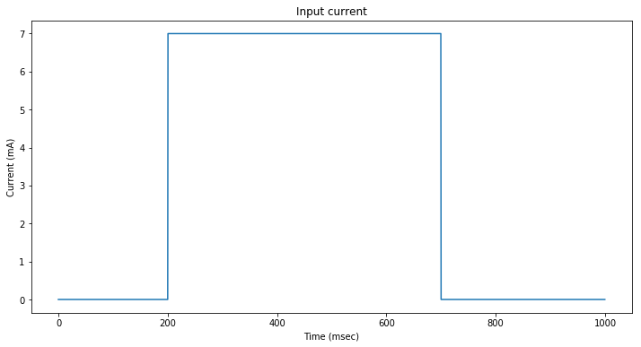
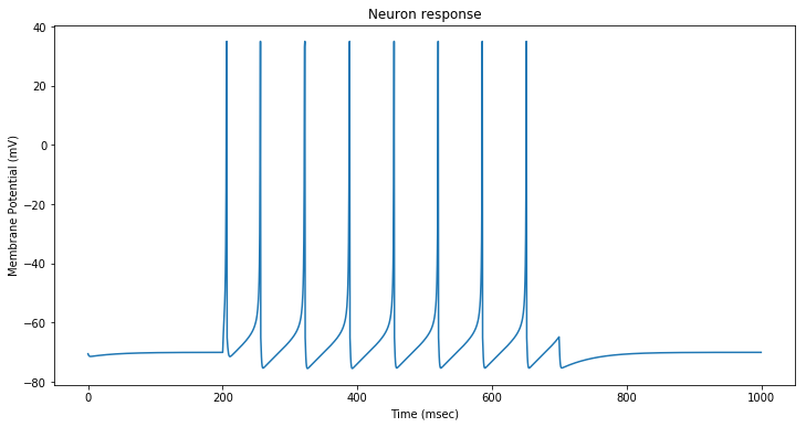
The neuron spikes at regular intervals. After each spike, the neuron membrane goes to its resting potential before starting to increase again.

Step 2: Simulate a single neuron with synaptic input

It is a simple variation of the previous experiment, where the input current is the composition of currents coming from several synapses (typically here, a hundred).

The formula for evaluating the synaptic current corresponds to the weighted sum of the input current generated by each synapse:

The current $Isyn(j)$ generated by each synapse is the multiplication of:

• a linear response to the membrane potential, with a target objective of potential $E_{in}(j)$: ($E_{in}(j) -v$)
• a conductance dynamics parameter, that is an exponential function $g_{in}(j)$ that is defined by a differential equation.

Each input synapse emits a spike following a poisson distribution of frequency $frate$. The probability that a neuron fires during the time interval $dt$ is thus $frate.dt$.

To simulate the neuron, we draw random numbers r in the $[0,1]$ interval at each timestep, and is the number $r$ is less than $frate.dt$, we generate a synapse spike by increasing the conductance dynamics for that synapse:

The complete synaptic current formula at each timestep is:

The corresponding Tensorflow code looks like this (see the jupyter notebook for details):

# First, update synaptic conductance dynamics:
# - increment by one the current factor of synapses that fired
# - decrease by tau the conductance dynamics in any case
g_in_update_op = tf.where(self.syn_has_spiked,
                          tf.add(self.g_in, tf.ones(shape=self.g_in.shape)),
                          tf.subtract(self.g_in, tf.multiply(self.dt,tf.divide(self.g_in, self.tau))))

# Update the g_in variable
g_in_op = tf.assign(self.g_in, g_in_update_op)

# We can now evaluate the synaptic input currents
# Isyn = Σ w_in(j)g_in(j)E_in(j) - (Σ w_in(j)g_in(j)).v(t)
i_op = tf.subtract(tf.einsum('nm,m->n', tf.constant(self.W_in), tf.multiply(g_in_op, tf.constant(self.E_in))),
                   tf.multiply(tf.einsum('nm,m->n', tf.constant(self.W_in), g_in_op), v_op))

We stimulate a neuron with $100$ synapses firing at $2 Hz$ between $200$ and $700 ms$.

Every millisecond, there are $0.001 * 2 * 100 = 0.2$ synapse spikes as an average.

In other words, a synapse spike occurs every $5 ms$ as an average.

The resulting membrane potential is displayed below:

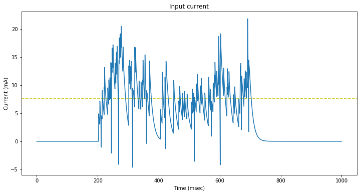
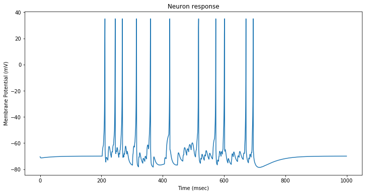
The synaptic input current oscillates around a mean value of approximately $10 mA$.

Due to the increased input current, the neuron spikes faster than in the previous stimulation.

Step 3: Simulate 1000 neurons with synaptic input

Each neuron is either:

• an inhibitory fast-spiking neuron $(a=0.1, d=2.0)$,
• or an excitatory regular spiking neuron $(a=0.02, d=8.0)$.

with a proportion of $20$ % inhibitory.

We therefore define a random uniform vector p on $[0,1]$, and condition the a and d vectors of our neuron population on p.

Each neuron is randomly connected with $10$ % of the input synapses, and thus receives an input synapse spike every $50 ms$ as an average.

Instead of displaying the membrane potentials, we just plot the neuron spikes for inhibitory (blue) and excitatory (yellow) neurons:

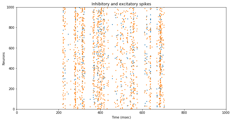
The neurons spike in ‘stripes’ at somehow regular intervals, with a bit of dispersion.

The neuron dynamics seem to act as a regulator to the synaptic ‘noise’.

Step 4: Simulate 1000 neurons with recurrent connections

A neuron i is sparsely (with probability $prc = 0.1$) connected to a neuron j.

Thus neuron i receives an additional current $Isyn(i)$ of the same form as the synaptic input:

The corresponding Tensorflow code looks like this (see the jupyter notebook for details):

# First, update recurrent conductance dynamics:
# - increment by one the current factor of synapses that fired
# - decrease by tau the conductance dynamics in any case
g_update_op = tf.where(has_fired_op,
                       tf.add(self.g, tf.ones(shape=self.g.shape)),
                       tf.subtract(self.g, tf.multiply(self.dt, tf.divide(self.g, self.tau))))
        
# Update the g variable
g_op = tf.assign(self.g, g_update_op)

# We can now evaluate the recurrent conductance
# I_rec = Σ wjgj(Ej -v(t))
i_rec_op = tf.einsum('ij,j->i', tf.constant(self.W), tf.multiply(g_op, tf.subtract(tf.constant(self.E), v_op)))

# Get the synaptic input currents from parent
i_in_op = super(SimpleSynapticRecurrentNeurons, self).get_input_ops(has_fired_op, v_op)
        
# The actual current is the sum of both currents
i_op = i_in_op + i_rec_op

Weights $w$ are Gamma distributed (scale $0.003$, shape $2$).

Inhibitory to excitatory connections are twice as strong.

$E(j)$ is set to $-85$ for inhibitory neurons, $0$ otherwise.

We again plot the neuron spikes for inhibitory (blue) and excitatory (yellow) neurons:

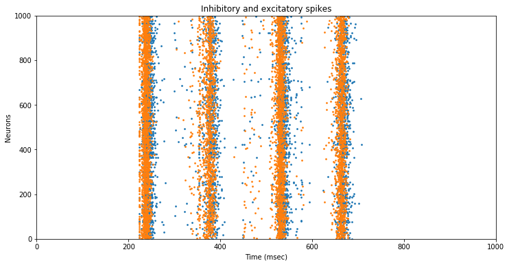
The addition of recurrent connections has drastically reduced the dispersion of the neuron spikes.