Identify Repeating Patterns using Spiking Neural Networks in Tensorflow
26 Jul 2018 by David CorvoysierSpiking neural networks (SNN) are the 3rd generation of neural networks.
SNN do not react on each stimulus, but rather accumulate inputs until they reach a threshold potential and generate a ‘spike’.
Because of their very nature, SNNs cannot be trained like 2nd generation neural networks using gradient descent.
Spike Timing Dependent Plasticity (STDP) is a biological process that inspired an unsupervised training method for SNNs.
In this article, I will provide an illustration of how STDP can be used to teach a single neuron to identify a repeating pattern in a continuous stream of input spikes.
For this, I will reproduce the STDP experiments described in Masquelier & Thorpe (2008) using Tensorflow instead of Matlab.
LIF neuron model
The LIF neuron model used in this experiment is based on Gerstner’s Spike Response Model.
At every time-step, the neuron membrane potential p is given by the formula:
\[p=\eta(t-t_{i})\sum_{j|t_{j}>t_{i}}{}w_{j}\varepsilon(t-t_{j})\]where $\eta(t-t_{i})$ is the membrane response after a spike at time $t_{i}$:
\[\eta(t-t_{i})=K_{1}exp(-\frac{t-t_{i}}{\tau_{m}})-K_{2}(exp(-\frac{t-t_{i}}{\tau_{m}})-exp(-\frac{t-t_{i}}{\tau_{s}}))\]and $\varepsilon(t)$ describes the Excitatory Post-Synaptic Potential of each synapse spike at time $t_{j}$:
\[\varepsilon(t-t_{j})=K(exp(-\frac{t-t_{j}}{\tau_{m}})-exp(-\frac{t-t_{j}}{\tau_{s}}))\]Note that K has to be chosen so that the max of $\eta(t)$ is 1, knowing that $\eta(t)$ is maximum when: \(t=\frac{\tau_{m}\tau_{s}}{\tau_{m}-\tau_{s}}ln(\frac{\tau_{m}}{\tau_{s}})\)
In this simplified version of the neuron, the synaptic weights $w_{j}$ remain constant.
The main graph operations are described below (please refer to my jupyter notebook for details):
    # Excitatory post-synaptic potential (EPSP)
    def epsilon_op(self):

        # We only use the negative value of the relative spike times
        spikes_t_op = tf.negative(self.t_spikes)

        return self.K *(tf.exp(spikes_t_op/self.tau_m) - tf.exp(spikes_t_op/self.tau_s))

    # Membrane spike response
    def eta_op(self):

        # We only use the negative value of the relative time
        t_op = tf.negative(self.last_spike)

        # Evaluate the spiking positive pulse
        pos_pulse_op = self.K1 * tf.exp(t_op/self.tau_m)

        # Evaluate the negative spike after-potential
        neg_after_op = self.K2 * (tf.exp(t_op/self.tau_m) - tf.exp(t_op/self.tau_s))

        # Evaluate the new post synaptic membrane potential
        return self.T * (pos_pulse_op - neg_after_op)

    # Neuron behaviour during integrating phase (t_rest = 0)
    def w_epsilons_op(self):

        # Evaluate synaptic EPSPs. We ignore synaptic spikes older than the last neuron spike
        epsilons_op = tf.where(tf.logical_and(self.t_spikes >=0, self.t_spikes < self.last_spike - self.tau_rest),
                               self.epsilon_op(),
                               self.t_spikes*0.0)

        # Agregate weighted incoming EPSPs
        return tf.reduce_sum(self.w * epsilons_op)
   ...
   def default_op(self):

        # Update weights
        w_op = self.default_w_op()

        # By default, the membrane potential is given by the sum of the eta kernel and the weighted epsilons
        with tf.control_dependencies([w_op]):
            return self.eta_op() + self.w_epsilons_op()

    def integrating_op(self):

        # Evaluate the new membrane potential, integrating both synaptic input and spike dynamics
        p_op = self.eta_op() + self.w_epsilons_op()

        # We have a different behavior if we reached the threshold
        return tf.cond(p_op > self.T,
                       self.firing_op,
                       self.default_op)

    def get_potential_op(self):

        # Update our internal memory of the synapse spikes (age older spikes, add new ones)
        update_spikes_op = self.update_spikes_times()

        # Increase the relative time of the last spike by the time elapsed
        last_spike_age_op = self.last_spike.assign_add(self.dt)

        # Update the internal state of the neuron and evaluate membrane potential
        with tf.control_dependencies([update_spikes_op, last_spike_age_op]):
            return tf.cond(self.t_rest > 0.0,
                           self.resting_op,
                           self.integrating_op)
Stimulate neuron with predefined synapse input
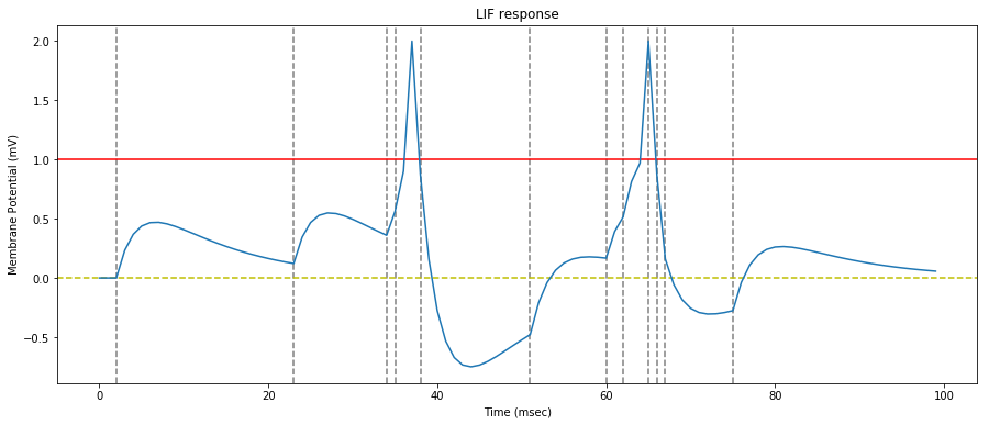
We replicate the $figure\,3$ of the original paper by stimulating a LIF neuron with six consecutive synapse spikes (dotted gray lines on the figure).
The neuron has a refractory period of $1\,ms$ and a threshold of $1$.
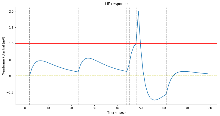
As in the original paper. we see that because of the leaky nature of the neuron, the stimulating spikes have to be nearly synchronous for the threshold to be reached.
Generate Poisson spike trains with varying rate
The original paper uses Poisson spike trains with a rate varying in the $[0, 90]\,Hz$ interval, with a variation speed that itself varies in the $[-1800, 1800]\,Hz$ interval (in random uniform increments in the $[-360,360]$ interval).
Optionally, we may force each synapse to spike at least every $\Delta_{max}\,ms$.
Please refer to my jupyter notebook for the details of the Spike trains generator.
We test our spike trains generator and draw the corresponding spikes. Both sets of spike trains use varying rates in the $[0, 90]\,Hz$ interval. The second set imposes $\Delta_{max}=50\,ms$.
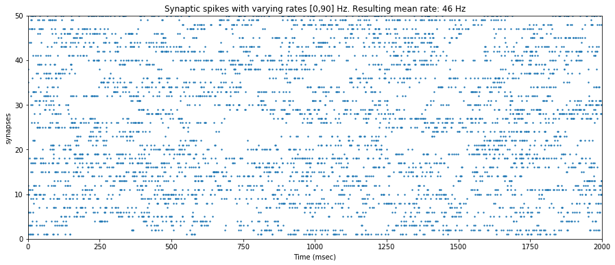
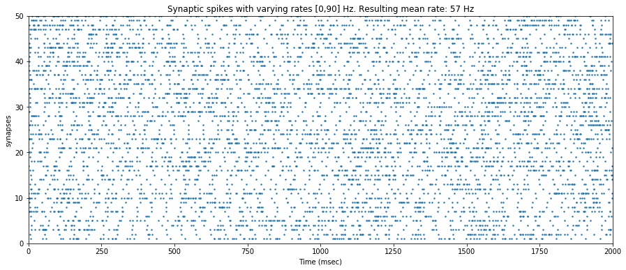
We note the increased mean rate of the second set of spike trains, due to the minimum $20\,Hz$ rate we impose (ie the maximum interval we allow between two spikes is $50\,ms$).
Stimulate a LIF Neuron with random spike trains
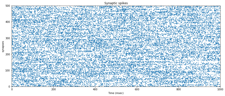
We now feed the neuron with $500$ synapses that generate spikes at random interval with varying rates.
The synaptic efficacy weights are arbitrarily set to $0.475$ and remain constant throughout the simulation.
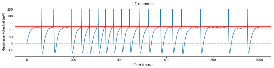
We draw the neuron membrane response to the $500$ random synaptic spike trains.
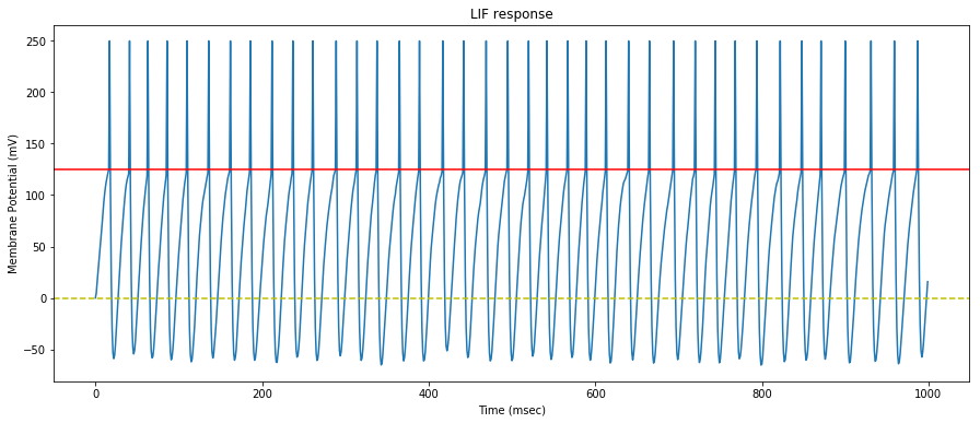
We can see that the neuron mostly saturates and continuously generates spikes.
Introduce Spike Timing Dependent Plasticity
We extend the LIFNeuron by allowing it to modify its synapse weights using a Spike Timing Dependent Plasticity algorithm (STDP).
The STDP algorithm rewards synapses where spikes occurred immediately before a neuron spike, and inflicts penalties to the synapses where spikes occur after the neuron spike.
The ‘rewards’ are called Long Term synaptic Potentiation (LTP), and the penalties Long Term synaptic Depression (LTD).
For each synapse that spiked $\Delta{t}$ before a neuron spike:
\[\Delta{w} = a^{+}exp(-\frac{\Delta{t}}{\tau^{+}})\]For each synapse that spikes $\Delta{t}$ after a neuron spike:
\[\Delta{w} = -a^{-}exp(-\frac{\Delta{t}}{\tau^{-}})\]As in the original paper, we only apply LTP, resp. LTD to the first spike before, resp. after a neuron spike on each synapse.
The main STDP graph operations are described below (please refer to my jupyter notebook for details:
    # Long Term synaptic Potentiation
    def LTP_op(self):

        # We only consider the last spike of each synapse from our memory
        last_spikes_op = tf.reduce_min(self.t_spikes, axis=0)

        # Reward all last synapse spikes that happened after the previous neutron spike
        rewards_op = tf.where(last_spikes_op < self.last_spike,
                              tf.constant(self.a_plus, shape=[self.n_syn]) * tf.exp(tf.negative(last_spikes_op/self.tau_plus)),
                              tf.constant(0.0, shape=[self.n_syn]))

        # Evaluate new weights
        new_w_op = tf.add(self.w, rewards_op)

        # Update with new weights clamped to [0,1]
        return self.w.assign(tf.clip_by_value(new_w_op, 0.0, 1.0))

    # Long Term synaptic Depression
    def LTD_op(self):

        # Inflict penalties on new spikes on synapses that have not spiked
        # The penalty is equal for all new spikes, and inversely exponential
        # to the time since the last spike
        penalties_op = tf.where(tf.logical_and(self.new_spikes, tf.logical_not(self.syn_has_spiked)),
                                tf.constant(self.a_minus, shape=[self.n_syn]) * tf.exp(tf.negative(self.last_spike/self.tau_minus)),
                                tf.constant(0.0, shape=[self.n_syn]))

        # Evaluate new weights
        new_w_op = tf.subtract(self.w, penalties_op)

        # Update the list of synapses that have spiked
        new_spikes_op = self.syn_has_spiked.assign(self.syn_has_spiked | self.new_spikes)

        with tf.control_dependencies([new_spikes_op]):
            # Update with new weights clamped to [0,1]
            return self.w.assign(tf.clip_by_value(new_w_op, 0.0, 1.0))
Test STDP with predefined input
We apply the same predefined spike train to an STDP capable LIFNeuron with a limited number of synapses, and draw the resulting rewards (green) and penalties (red).
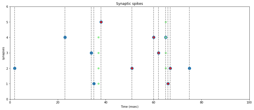
On the graph above, we verify that the rewards (green dots) are assigned only when the neuron spikes, and that they are assigned to synapses where a spike occured before the neuron spike (big blue dots).
Note: a reward is assigned event if the synapse spike is not synchronous with the neuron spike, but it will be lower.
We also verify that a penaly (red dot) is inflicted on every synapse where a first spike occurs after a neuron spike.
Note: these penalties may later be counter-balanced by a reward if a neuron spike closely follows.
Stimulate an STDP LIF Neuron with random spike trains
The goal here is to check the effects of the STDP learning on the neuron behaviour when it is stimulated with our random spike trains.
We test the neuron response with three set of spike trains, with a mean rate of $35$, $45$ and $55$ $Hz$ respectively.
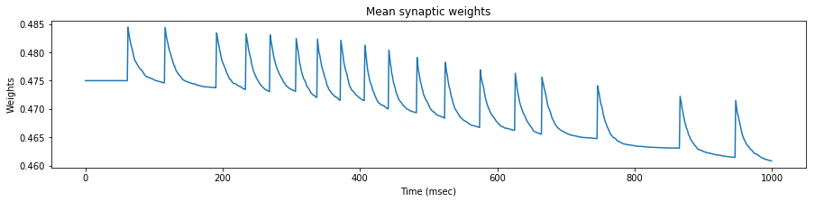
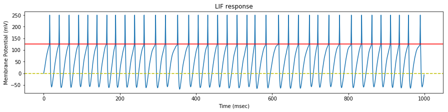
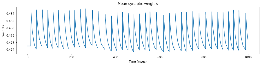
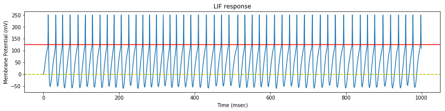
We see that the evolution of the synapse weights as a response to this steady stimulation is highly dependent of the mean input frequency.
If the mean input frequency is too low, the neuron exhibits a low decrease of the synaptic efficacy weights, down to the point where the neuron is not able to fire anymore.
If the mean input frequency is too high, the neuron exhibits in the contrary an increase of the synaptic efficacy weights, up to the point where it fires regardless of the input.
Using the STDP values of the original paper, only the exact mean frequency of $45$ $Hz$ (the one also used in the paper) exhibits some kind of stability.
As a conclusion, either our implementations differ, or the adverse effect of this particular STDP algorithm has been overlooked in the original paper, because as we will see later, the actual mean stimulation rate will be around $64$ $Hz$.
Generate recurrent spike trains
We don’t follow exactly the same procedure as in the original paper, as the evolution of the hardware and software allows us to generate spike trains more easily. The result, however, is equivalent.
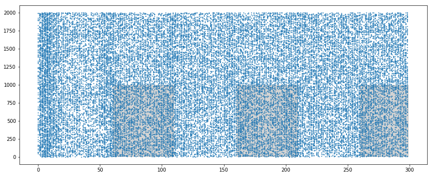
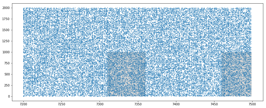
We generate $2000$ spike trains, from which we force the $1000$ first to repeat a $50\,ms$ pattern at random intervals.
The time to the next pattern is chosen with a probability of $0.25$ among the next slices of $50\,ms$ (omitting the first one to avoid consecutive patterns).
We display the resulting synapse mean spiking rates, and some samples of the spike trains, identifying the pattern (gray areas).
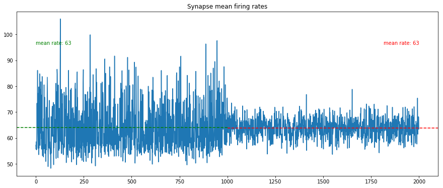
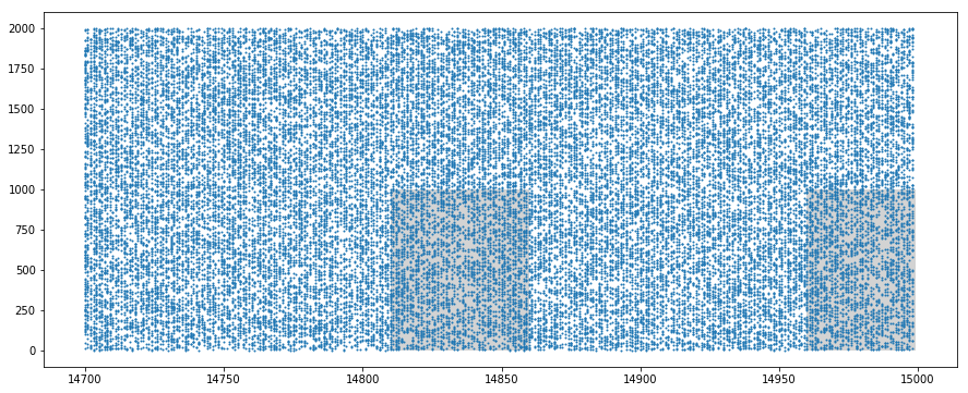
We verify that the mean spiking rate is the same for both population of synapses (approximately $64\,Hz = 54\,Hz + 10\,Hz$).
We nevertheless notice that the standard deviation is much higher for the synapses involved in the pattern.
On the spike trains samples, one can visually recognize the patterns thanks to the gray background, but otherwise they would go unnoticed for the human eye.
We also verify that each pattern is slightly modified by the $10\,Hz$ spontaneous activity.
Stimulate an STDP LIF neuron with recurrent spiking trains
We perform a simulation on our STDP LIF neuron with the generated spike trains, and draw the neuron response at the begining, middle and end of the simulation.
On each sample, we identify the pattern interval with a gray background.
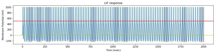
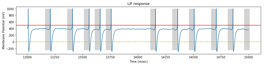
At the beginning of the stimulation, the neuron spikes continuously, inside and outside the pattern.
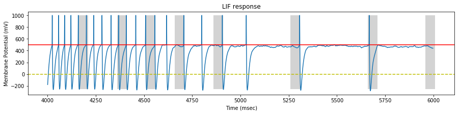
At the middle of the stimulation, the neuron fires mostly inside the pattern and sometimes outside the pattern (false positive).
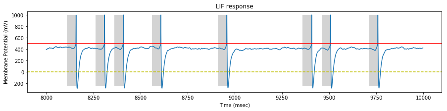
At the end of the stimulation, the neuron fires only inside the pattern.
Important note: With the rates specified in the original paper, the neuron quickly saturates and doesn’t learn anything. With a tweaked LTD factor $a^{-}$, that seems to be dependent of the spike trains, the neuron learns the pattern after only a few seconds of presentation: Hurray ! For a given set of spike trains, you might adjust the rate to achieve a successful training
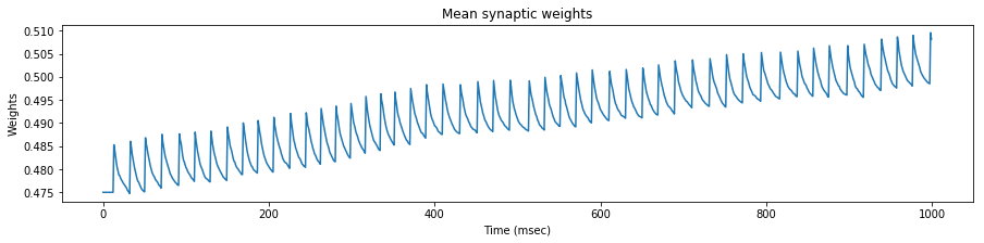
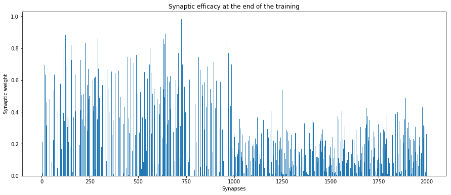
The neuron has become more an more selective as the pattern presentation were repeated, up to the point where the synapses involved in the pattern have dominant weights, as displayed on the graph below.
Discussion
We managed to reproduce the experiments described in Masquelier & Thorpe (2008) using Tensorflow.
However, we found out that the STDP parameters needed to be tweaked to adjust to the input spike train mean rate, and possibly also to adjust to the generated spike trains themselves, as for a given rate, the neuron did not react identically for different sets of spike trains.
Also, we found out that the neuron doesn’t necessarily identify the beginning of the pattern, but sometime its end.
These differences with the original paper raise questions about the differences between our implementation and the original one done in Matlab.
comments powered by Disqus