Leaky Integrate and Fire neuron with Tensorflow

Spiking Neural Networks (SNN) are the next generation of neural networks, that operate using spikes, which are discrete events that take place at points in time, rather than continuous values.

Essentially, once a stimulated neuron reaches a certain potential, it spikes, and the potential of that neuron is reset.

In this article, I will detail how the Leaky Integrate and Fire (LIF) spiking neuron model can be implemented using Tensorflow.

Leaky-integrate-and-fire model

We use the model described in § 4.1 of “Spiking Neuron Models”, by Gerstner and Kistler (2002).

The leaky integrate-and-fire (LIF) neuron is probably one of the simplest spiking neuron models, but it is still very popular due to the ease with which it can be analyzed and simulated.

The basic circuit of an integrate-and-fire model consists of a capacitor C in parallel with a resistor R driven by a current I(t):

The driving current can be split into two components, $I(t) = IR + IC$.

The first component is the resistive current $IR$ which passes through the linear resistor $R$.

It can be calculated from Ohm’s law as $IR = \frac{u}{R}$ where $u$ is the voltage across the resistor.

The second component $IC$ charges the capacitor $C$.

From the definition of the capacity as $C = \frac{q}{u}$ (where $q$ is the charge and $u$ the voltage), we find a capacitive current $IC = C\frac{du}{dt}$. Thus:

By multiplying the equation by $R$ and introducing the time constant $\tau_{m} = RC$ this yields the standard form:

where $u(t)$ represents the membrane potential at time $t$, $\tau_{m}$ is the membrane time constant and $R$ is the membrane resistance.

When the membrane potential reaches the spiking threshold $u_{thresh}$, the neuron ‘spikes’ and enters a resting state for a duration $\tau_{rest}$.

During the resting perdiod the membrane potential remains constant a $u_{rest}$.

Step 1: Create a single LIF model

In a first step, we create a tensorflow graph to evaluate the membrane response of a LIF neuron.

For encaspulation and isolation, the graph is a member of a LIFNeuron object that takes all model parameters at initialization.

The LIFNeuron object exposes the membrane potential Tensorflow ‘operation’ as a member.

The input current and considered time interval are passed at Tensorflow placeholders.

The main graph operations are described below (please refer to my jupyter notebook for details:

    # Neuron behaviour during integration phase (below threshold)
    def get_integrating_op(self):

        # Get input current
        i_op = self.get_input_op()

        # Update membrane potential
        du_op = tf.divide(tf.subtract(tf.multiply(self.r, i_op), self.u), self.tau) 
        u_op = self.u.assign_add(du_op * self.dt)
        # Refractory period is 0
        t_rest_op = self.t_rest.assign(0.0)
        
        with tf.control_dependencies([t_rest_op]):
            return u_op

    # Neuron behaviour during firing phase (above threshold)    
    def get_firing_op(self):                  

        # Reset membrane potential
        u_op = self.u.assign(self.u_rest)
        # Refractory period starts now
        t_rest_op = self.t_rest.assign(self.tau_rest)

        with tf.control_dependencies([t_rest_op]):
            return u_op

    # Neuron behaviour during resting phase (t_rest > 0)
    def get_resting_op(self):

        # Membrane potential stays at u_rest
        u_op = self.u.assign(self.u_rest)
        # Refractory period is decreased by dt
        t_rest_op = self.t_rest.assign_sub(self.dt)
        
        with tf.control_dependencies([t_rest_op]):
            return u_op

    def get_potential_op(self):
        
        return tf.case(
            [
                (self.t_rest > 0.0, self.get_resting_op),
                (self.u > self.u_thresh, self.get_firing_op),
            ],
            default=self.get_integrating_op
        )

Step 2: Stimulation by a square input current

We stimulate the neuron with three square input currents of vaying intensity: 0.5, 1.2 and 1.5 mA.

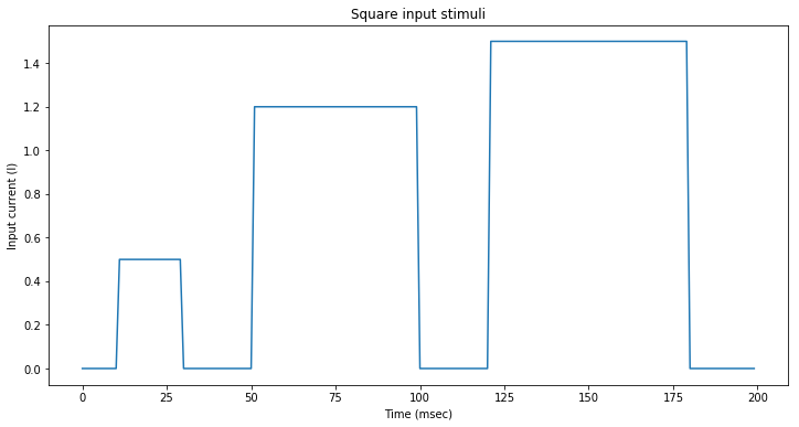
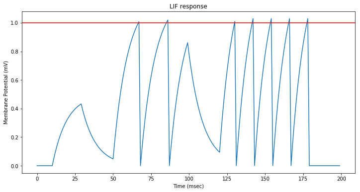
The first current step is not sufficient to trigger a spike. The two other trigger several spikes whose frequency increases with the input current.

Step 3: Stimulation by a random varying input current

We now stimulate the neuron with a varying current corresponding to a normal distribution of mean 1.5 mA and standard deviation 1.0 mA.

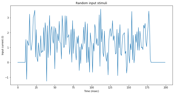
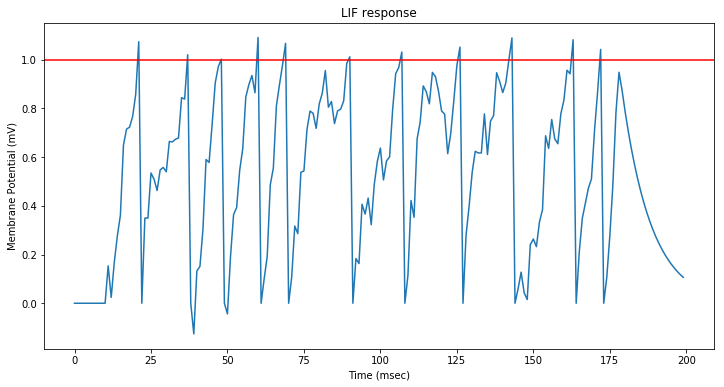
The input current triggers spike at regular intervals: the neuron mostly saturates, each spike being separated by the resting period.

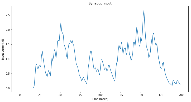
Step 4: Stimulate neuron with synaptic currents

We now assume that the neuron is connected to input neurons through $m$ synapses.

The contribution of the synapses to the neuron input current is given by the general formula below:

Where $t_i^{(f)}$ is the time of the f-th spike of the synapse $i$.

A typical implementation of the $I_{syn}$ function is:

where $q$ is the total charge that is injected in a postsynaptic neuron via a synapse with efficacy $w_{j} = 1$.

Note that $\frac{dI_{syn}}{dt}=-\frac{I_{syn}(t)}{\tau}$.

We create a new neuron model derived from the LIFNeuron.

The graph for this neuron includes a modified operation to evaluate the input current at each time step based on a memory of synaptic spikes.

The graph requires a new boolean Tensorflow placeholder that contains the synapse spikes over the last time step.

The modified operation is displayed below (please refer to my jupyter notebook for details:

    # Override parent get_input_op method
    def get_input_op(self):
        
        # Update our memory of spike times with the new spikes
        t_spikes_op = self.update_spike_times()

        # Evaluate synaptic input current for each spike on each synapse
        i_syn_op = tf.where(t_spikes_op >=0,
                            self.q/self.tau_syn * tf.exp(tf.negative(t_spikes_op/self.tau_syn)),
                            t_spikes_op*0.0)

        # Add each synaptic current to the input current
        i_op =  tf.reduce_sum(self.w * i_syn_op)
        
        return tf.add(self.i_app, i_op)     

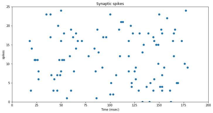
Each synapse spikes according to an independent poisson process at $\lambda = 20 hz$.

We perform a simulation by evaluating the contribution of each synapse to the input current over time.

At every time step, we draw a single sample $r$ from a uniform distribution in the $[0,1]$ interval, and if it is lower than the probability of a spike over the time interval (ie $r < \lambda.dt$) then a spike occurred.

Note that this assumes that the chosen time interval is lower than the minimum synapse spiking interval.

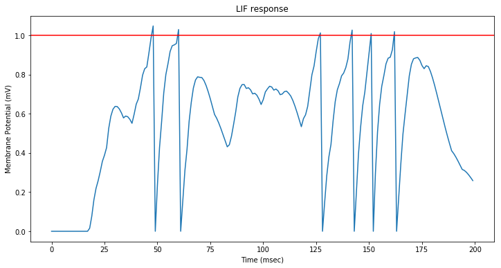
As expected, the neuron spikes when several synapses spike together.